Simple Linear Regression
Notes and Ideas:
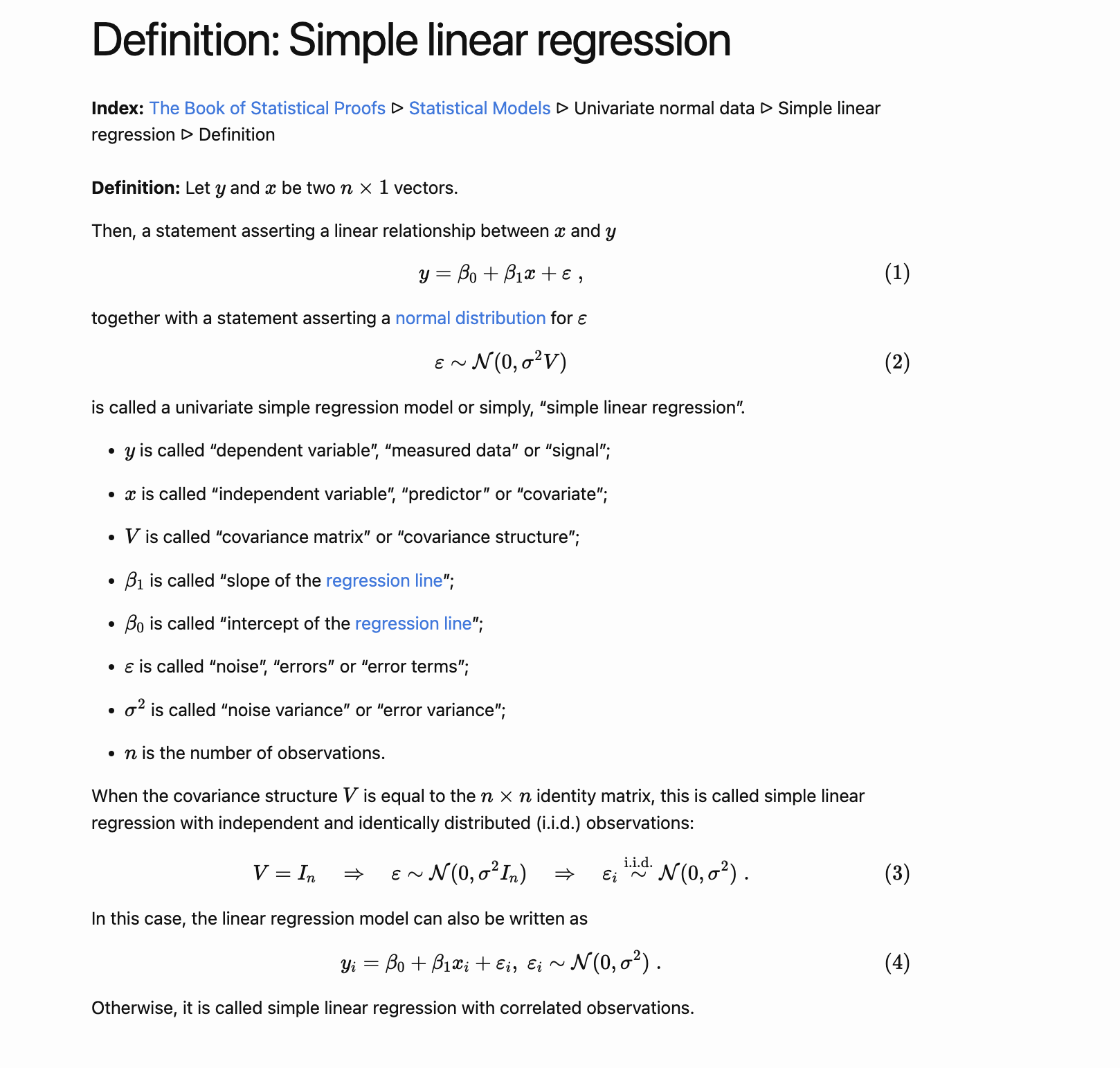
Model Setup:
True Model:
: observed value of the response variable Y of the observation : observed value of the independent variable x of the observation - n: sample size
and : unknown fixed coeffcient parameters — constant : Random Error term -cosntant
simple: only one explanatory variable
Linear: linear in the parameters
The slope is denoted by
note: linear:
Linear vs Non Linear
Example for linear equation:
House Price = Intercept + Coefficient * Square Footage
Example for non-linear equation:
Population Growth = A * Time^B
In both examples, linear regression assumes a straight-line relationship between variables, while nonlinear regression introduces more complex equations that capture nonlinear patterns
Link to original
Linear vs Non Linear
Example for linear equation:
House Price = Intercept + Coefficient * Square Footage
Example for non-linear equation:
Population Growth = A * Time^B
In both examples, linear regression assumes a straight-line relationship between variables, while nonlinear regression introduces more complex equations that capture nonlinear patterns
Link to originalModel Assumption:
is Random error term: - Estimation Assumptions:
- E(
)=0 - Var(
) = , for all i. (The errors have constant variance) unknown fixed parameter - Cov(
, ) = 0. (no correlation between errors for each observations, The errors are independent of each other) - Classic Assumption(Model Inference):
^The errors are normally distributed.
- E(
- Estimation Assumptions:
is also a fixed value affect to = -> estimate 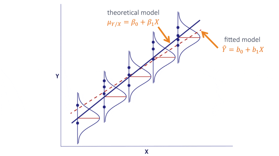
Model Estimation:
Goal:
MLE Approach:
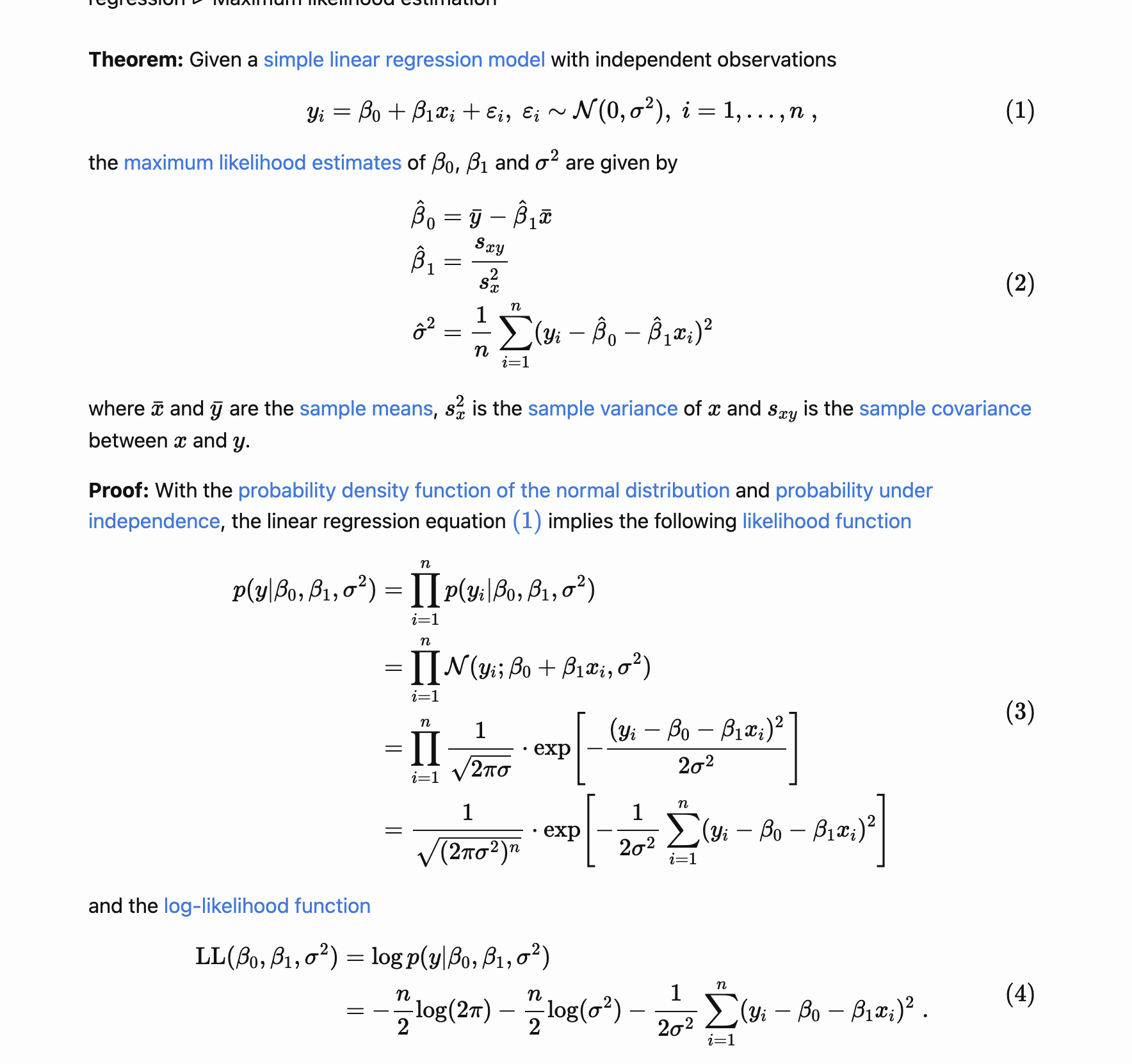
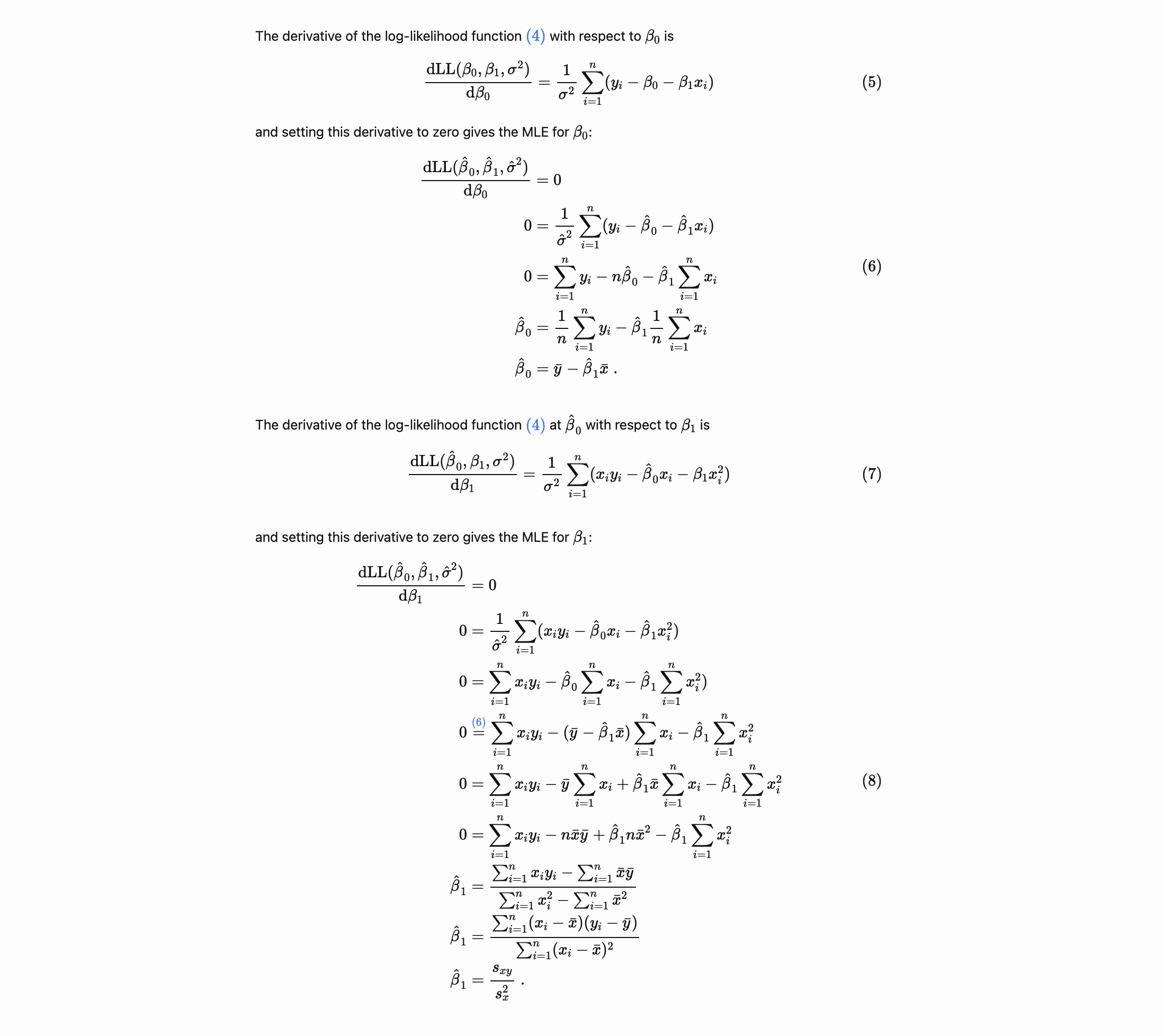
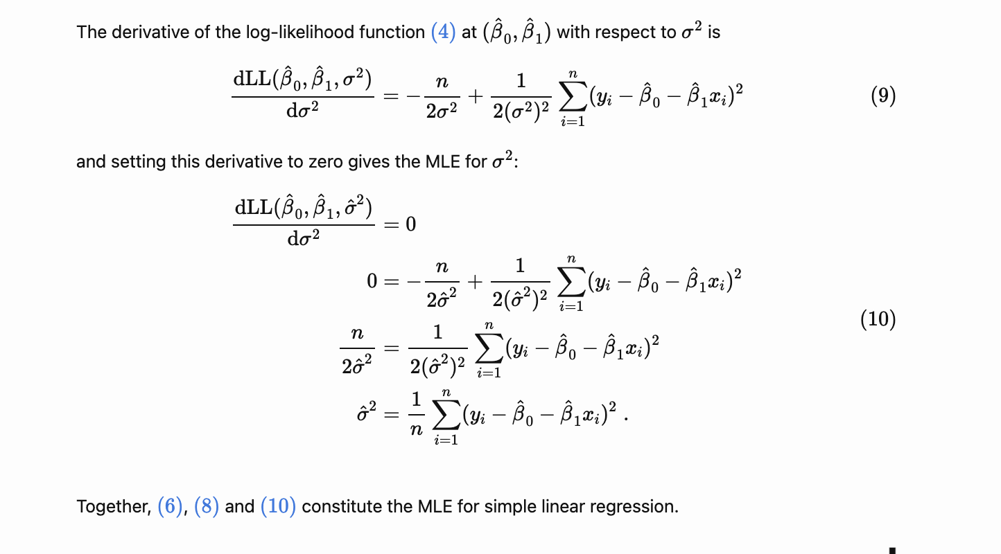
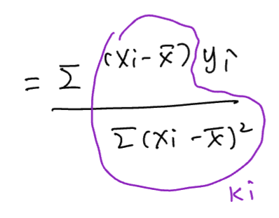
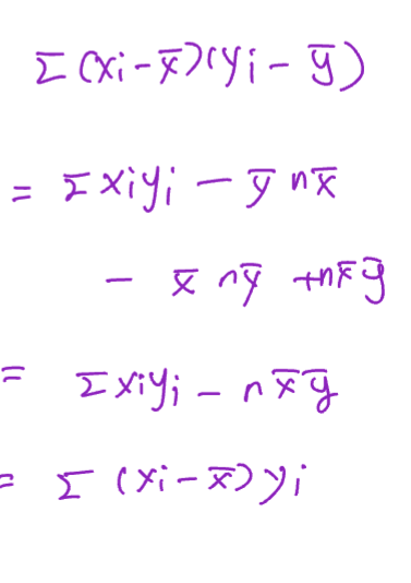
Ordinary Least Square Estimate(OLSE)
find
Note:
Example:
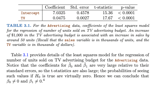
Example 1.1 Continued - Coffee Sales and Shelf Space For the coffee data, we observe the following summary statistics in Table 2. Table 2: Summary Calculations - Coffee sales data From this, we obtain the following sums of squares and crossproducts.
From these, we obtain the least squares estimate of the true linear regression relation
Gauss-Markov Theorm:
OLSE is the Best Linear Unbiased Estimators of
- Linear:
and are linear combinations of . - Best: OLSE has the smallest variance among all the linear estimators of
and
Proof:
from OLSE we got:
=>  =>
=>
note:
(i)
for variance
From OLSE we got:
-(a)
since
Thus we plug back to (a)
For variance of
The key assumptions (conditions) that need to be satisfied for the Gauss-Markov theorem to hold:
- Linearity in Parameters: The regression model is linear in parameters. In the context of a simple linear regression, this can be represented as
, where is the dependent variable, is the independent variable, and is the error term. - Random Sampling: The data (observations) are obtained using a random sampling process.
- No Perfect Collinearity: For the multiple regression case, no independent variable is a perfect linear function of other explanatory variables. In simple linear regression, this is trivially satisfied since there’s only one independent variable.
- Zero Conditional Mean: The expected value of the error term, given the independent variable(s), is zero. Mathematically, this is represented as
. This implies that any variation in the error term is not systematically related to the independent variable(s). - Homoscedasticity: The variance of the error term is constant across all values of the independent variable(s). Formally,
. This means that the spread of the residuals remains constant as the value of the independent variable(s) changes.
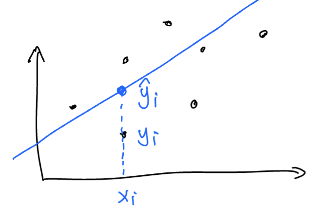
Fitted Value:
is an unbiased estimation of - When talking about
is an “estimation” of , we are talking about the distribution of the biased/error/residual =
 NOTE:
NOTE:
mean out of sample prediction - (1)
is an estinate of unbiased. Hint: - (2) when
is an “prediction” / “Estimation” of , we are talking about the sampling distribution of
Residuals
Residulas
Residulas
Notes and Ideas:
Defination:
- Residuals in a statistical or machine learning model are the differences between observed and predicted values of data. They are a diagnostic measure used when assessing the quality of a model. They are also known as errors
is an estimation of =0 . unbiased - Note:
is an unbiased estimator of - Sampling distribution of
:
Normally distributed
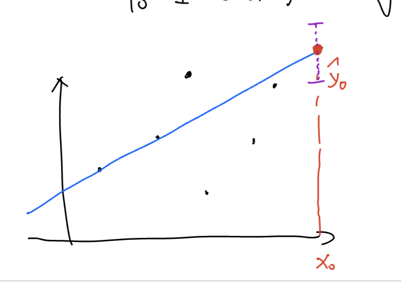
Out of Sample Error: given
(new data) properties: Sampling distribution of
:
- Normally Distribution
Use :
- Residuals are importatant when determining the quality of a model. We can examine residuals in terms of their mahnitude and/ or whether they form a parttern
- Where the residuals are all 0, the model predicts perfectly. THe further residuals are from 0, the less accurate the model. In the case of Linear Regression, the greater the sum of squared residucals, the smaller the r-squared tatistic, all else being equal
- Where the average residual is not 0, it implies that the model is systematically biased(i.e., consistently over-or under-predicting)
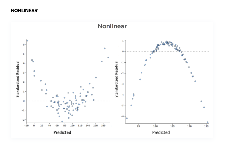
Residual plot:
- In the case of simple linear regression (regression with 1 predictor), we set the predictor as the x-axis and the residual as the y-axis
- In the case of multiple linear regression (regression with >1 predictor), we set the fitted value as the x-axis and the residual as the y-axis
Residcual function:
Properties:
- mean of the residuals should be 0
- Variance of e
- Non-independence, Scine
is normally distributed For simple linear regression(2D):
TAGS
Link to original
Estimate
Idea: for
a sample from
Calculate SSE
hint:
(with
Thus we have:
Mean Square Error(MSE):
MSE
Testing:
Testing for
Test set up:
Rejection Rule :
Reject
Anova and F test in SLR
Hint:
Anova Table
NOTE:
=> = when When - F test and t test are equavilent in SLR -> p-value of F = p-value of t, the test statistic relationship between t-test and F-test in the context of SLR is
F test is used to ocmpare a “shorter” model and a “longer model”:
Testing set up:
or
IN SLR:
<=>
note:
SSE-Reduced > SSE-FULL, Adding predictors to a linear regression model will always reduces SSE. RMSE always selects the model with most predictors
Lower values of RMSE indicate a better fit of the model to the data, while higher values indicate a poorer fit. However, by itself, RMSE doesn’t tell you whether the model’s predictions are biased. It merely indicates the magnitude of the error.
R-squared
Coefficient of Determination to measure the goodness of fit of a model.
The proportion of the variation in Y contained
note:
in SLR
Prediction intervals for predictions
let x =
Estimate
Confidence interval for estimating
Thus we have
Confident Interval for estimation of Bias
Prediction Interval for
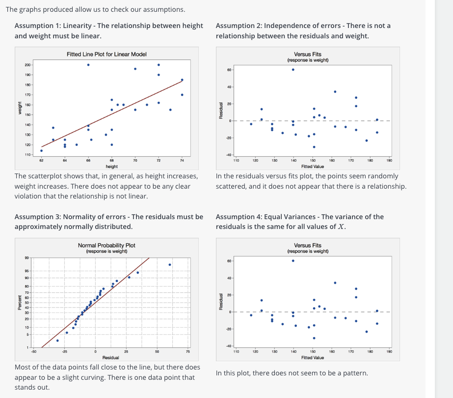
SEL Model Assumption Diagnosis:
Example