Author: Freeman Chen, John Ginos
Date: 2023-03-29
Stats 530
Abstract
This paper investigates the hypothesis that two particular amateur basketball players have greater shooting efficiency when shooting a basketball on the side of the basket associated with their shooting arm (in the case of the two participants, the right side of the basket). For each participant, data on shooting efficiency, measured as the time in seconds that it takes to make three baskets from a particular location on the court, are collected (the indicator variable determining the side of the basket the shooter is on is termed the shooter’s ‘orientation’). A multiple linear regression model is proposed and estimated where the key independent variable is the side of the basket the shot originates from (left or right). Other controls to capture location of the shooter on the court (and which shooter is being timed) are included in the model. Only the estimate for the parameter associated with the shooter’s distance to the basket is significant. Thus, it is concluded that there is not significant evidence in the data to suggest that the shooter’s orientation improves shooting efficiency. diagnostic tests on the model residuals are performed. While model residuals deviate significantly from normality and suggest the presence of heteroscedasticity, diagnostic tests reveal that is no evidence of autocorrelation in the residuals. Furthermore, the multicollinearity among the model predictors is examined and is determined not to be a major problem. Only one outlying observation is present in the data. Potential areas for future research and limitations of the analysis performed in this paper are discussed.
Data Collection
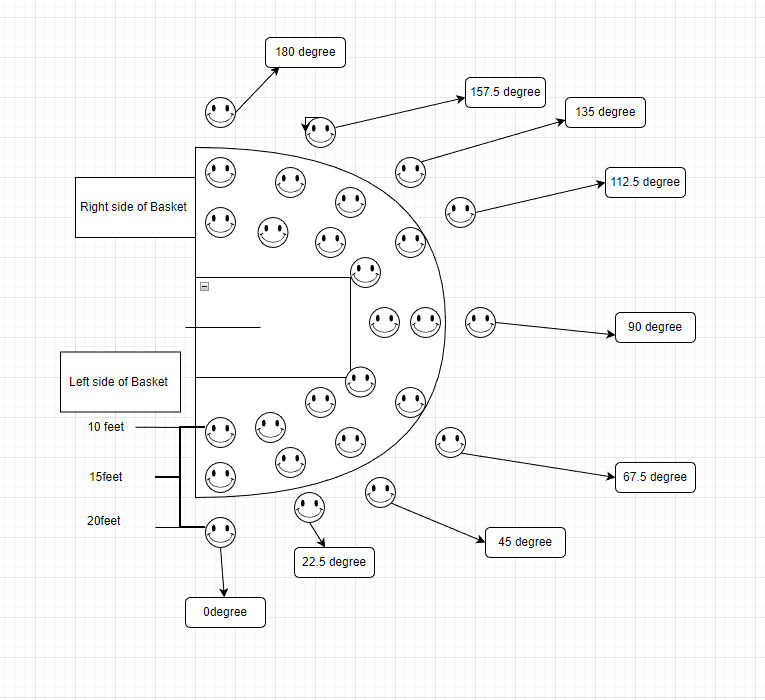 (Figure 1)
Positions on the court are marked based on their distance to the basket and the angle (in degrees) between the particular position and the baseline of the court (see Figure 1). Two amateur basketball players with experience shooting a basketball (in leisurely, non-competitive games of basketball or as personal, albeit infrequent, practice) are timed to see how long it takes them (measured in seconds) to make 3 baskets. While one player is engaged in shooting the basketball (while being timed by stopwatch), the other is rebounding the ball and returning it to the shooting player to avoid causing the shooting player wait for a ball between setting up for a shot or actively shooting (we call this time, down-time). Multiple basketballs are made available for the shooting player to avoid excessive down-time. The players take turns at each location. The first times are recorded for each player at the 10-foot distance and at an angle of zero degrees. This is the angle to the basket where the players are nearest the baseline (or out-of bounds line) and have almost no visibility of the front surface of the backboard; the players are facing a direction parallel to the baseline. Furthermore, at this angle, the players shoot with an orientation that is to the left of the basket. The players proceed to shoot at the 22.5, 45, 67.5, 90, 112.5, 135, 157.5, and 180-degree angles to the basket (see Figure 1) while maintaining the 10-foot distance. Once the players finish their shooting at the 10-foot distance and at an angle of 180 degrees, they begin from the 180-degree angle at the 15-foot distance and continue from there, taking turns recording data at each angle along the 15-foot distance.
Once they arrive back at the 0-degree angle and finish shooting at the 15-foot distance at that position, they repeat the pattern of shooting at each each angle in the order taken when they shot from the 10-foot distance but skip over the 67.5, 90, and 112.5 degree angles for sake of time. After the finishing shooting at the 180-degree angle, the shooters return to the 90-degree angle (at the 20-foot distance still) to finish collecting the data at that location. Note that neither player recorded shooting times at the 20-foot distance and at the 67.5 and 112.5-degree angles due to time limitations.
The choice of moving across the court in the fashion described (the players going to each angle at a fixed distance until each player shoots at each angle) is done to avoid the situation where the players take all shots on one side of the basket first and then, once they are ‘warmed up’, take shots on the other side of the basket. This would cause potential ‘warm-up’ bias in the data collection.
The person independent variable is an indicator variables where a 1 is recorded when John was shooting and a 0 is recorded when Freeman is shooting. Similarly, the orientation independent variable is an indicator variable with a 1 recorded for a left-sided orientation (including the 90-degree angle where the player shoots while facing the basket directly) and a 0 is recorded for a right-sided orientation.
Descriptive statistics based on the 50 observations within the data are provided for the recorded times (in seconds) and other independent variables associated with location on the court and the shooter.
CHART OF DESCRIPTIVE STATISTICS TABLE
Note that there appears to be a significant outlier in the dependent variable, time. This is obvious numerically as the interquartile range is 20.29 and the difference between the maximum value and the value of the 3rd quartile is 100.45. Thus, the data are evidently right-skewed.
A plot of shooting efficiency against Angle (with distance to basket given by color is given below)
EFFICIENCY BY ANGLE AND DISTANCE (COLOR) PLOT
.PNG)
Interestingly, there is a discernible pattern of increased variance for shooting efficiency at angles that belong to the left-sided orientation with the exception of the 90-degree angle (i.e. angles of 0-67.5 degrees). The plot also seems to reveal a potential difference in the mean shooting efficiency between angles below 90-degrees and angles equal to or greater than 90-degrees (one apparent outlier disrupts the pattern slightly). This will be formally measured by means of the multiple linear regression model.
It is also clear from the plot that there is much less variance in the shooting efficiency measurements at the 10-foot distance (red) compared with the measurements at the 20-foot distance (blue). This may indicate the fact that there may not be a relationship between the variance of the dependent variable and the independent variables.
RESULTS
The proposed model is given as
MODEL STATEMENT
SHOOTING EFFICIENCY =
The multiple linear regression model results are provided below
Residuals:
Coefficients:
ADJ R SQUARED AND F STATISTIC AND p-value:
Note that the parameter estimates, including the intercept term, are all statistically insignificant (at the 95% significance level) with the exception of the estimate associated with the distance independent variable. Therefore, the data do not give sufficient evidence to suggest that the two players in the study have greater shooting efficiency (lower shooting times) when shooting with a right-sided orientation. Because the only significant parameter estimate is the one associated with the distance variable, only an interpretation of the distance parameter is given.
The parameter estimate associated with the distance variable is approximately 2.82 suggesting that an increase in the distance by one foot is associated with an increase in the time it takes for a shooter to make 3 baskets or a decrease in the shooting efficiency of approximately 2.82 seconds. This is the expected association between distance and shooting efficiency.
The low R squared value suggests that the proposed model is not particularly effective at capturing variation in shooting efficiency. This may be due to other omitted variables and measurement error when measuring shooting times. However, the F-statistic is statistically significant at the 95% significance level, so we may conclude that there is indeed evidence that at least one of the parameters of the models is not zero.
DIAGNOSTICS
Model diagnostics are considered to assess the viability of the model.
A plot of the residuals of the model against the predicted values is given below.
PLOT OF RESIDUALS AGAINST PREDICTED
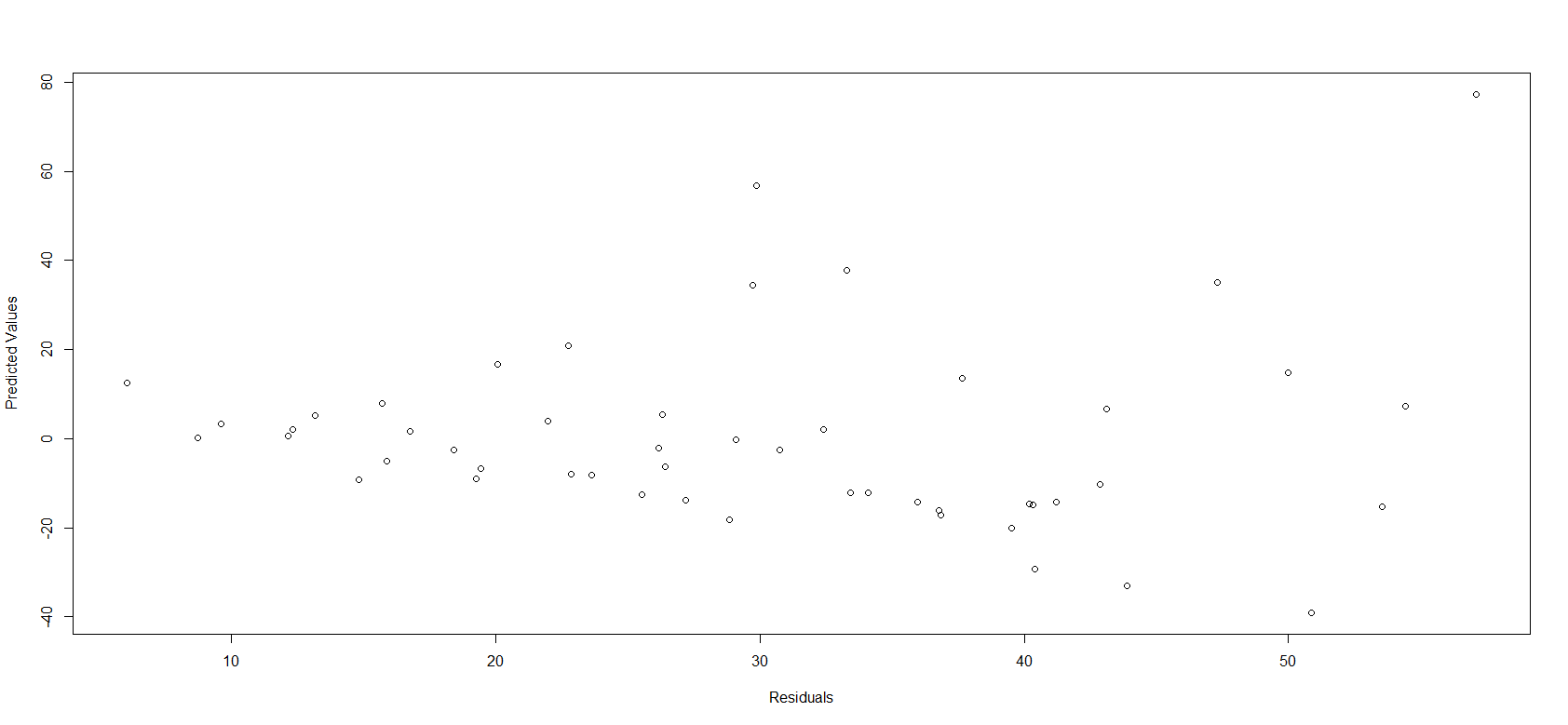
The residuals exhibit a pattern of near-perfect heteroscedasticity (the characteristic funnel shape appears to manifests itself in the model residuals). However, the Breusch-Pagan test has a p-value that is approximately 0.0562. Thus, while there is not have sufficient evidence to reject the null-hypothesis of homoscedasticity in the residuals (based on a 95% significance level), the p-value is close to the threshold of statistical significance and the plot reveals a concerning patter. Thus, the model estimates may be unreliable.
The data were collected in the order that they are analyzed so the index of the residuals represents the order of the residuals with respect to when the data were collected. A plot of the model residuals against the index of the residuals is given below.
PLOT OF RESIDUALS AGAINST INDEX
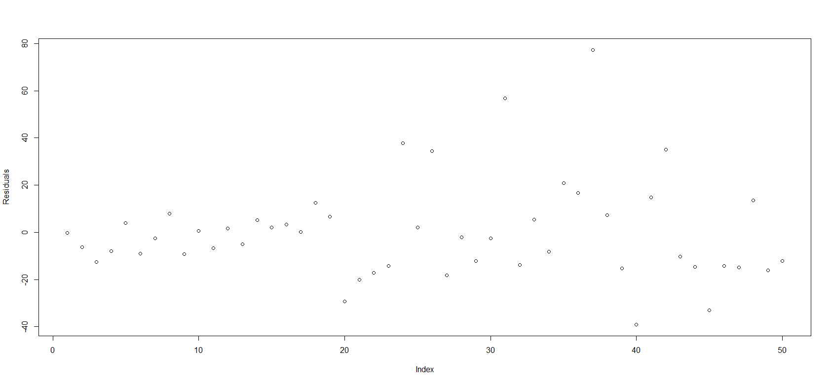
The plot reveals a largely random pattern in the residuals (increasing variance is likely due to the fact that the players shot from further distance toward the end of the experiment). The Durbin-Watson test confirms this. The test statistic is 1.7791 and the assocaited p-value is 0.1582, suggesting that there is not sufficient evidence to reject the null-hypothesis of an autocorrelation parameter of 0 for the residuals.
Next, the assumption of normality in the residuals is considered. The following normal probability plot demonstrates that the residuals appear to significantly deviate from normality in the upper quantiles of the empirical distribution.
NORMAL PROB PLOT AND QQLINE
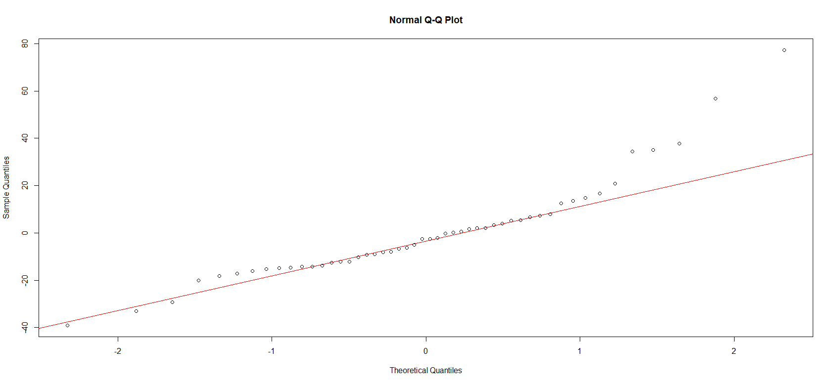
A two-sided Kolmogorov-Smirnov test yields a test statistic of D = 0.52561 and a p-value of approximately 0. Thus, it may concluded that there is sufficient evidence to suggest that the residuals are not normally distributed. Moreover, the p-value of the Shapiro-Wilk test for normality is 0.0002544 < 0.05 which confirms what the normal probability plot reveals.
To check the assumption of collinearity in the model predictors, the correlation matrix is obtained for the independent variables and the determinant is computed.
CORRELATION MATRIX
As expected, orientation and angle are highly correlation (since larger angles are considered to be on the right side of the basket, this could be avoided in future work by simply keeping the angles between 0 and 90 degrees and measuring the side of the basket using orientation only). The correlation coefficient for orientation and angle is about -0.88. Additionally, the determinant of the correlation matrix has an absolute value of about 0.23 suggesting that multicollinearity may be a slight problem. However, the variance inflation factors (vif’s) are computed for each independent variable and none are greater than 5, suggesting that multicollinearity is not a major problem. The calculated vif’s are given below.
VIF TABLE
Lastly, the studentized deleted residuals and hat values are computed to determine if outlying observations and/or influential observations are apparent in the data. A plot of the studentized delted residuals is given below.
PlOT OF STUDENTIZED DELETED RESIDUALS
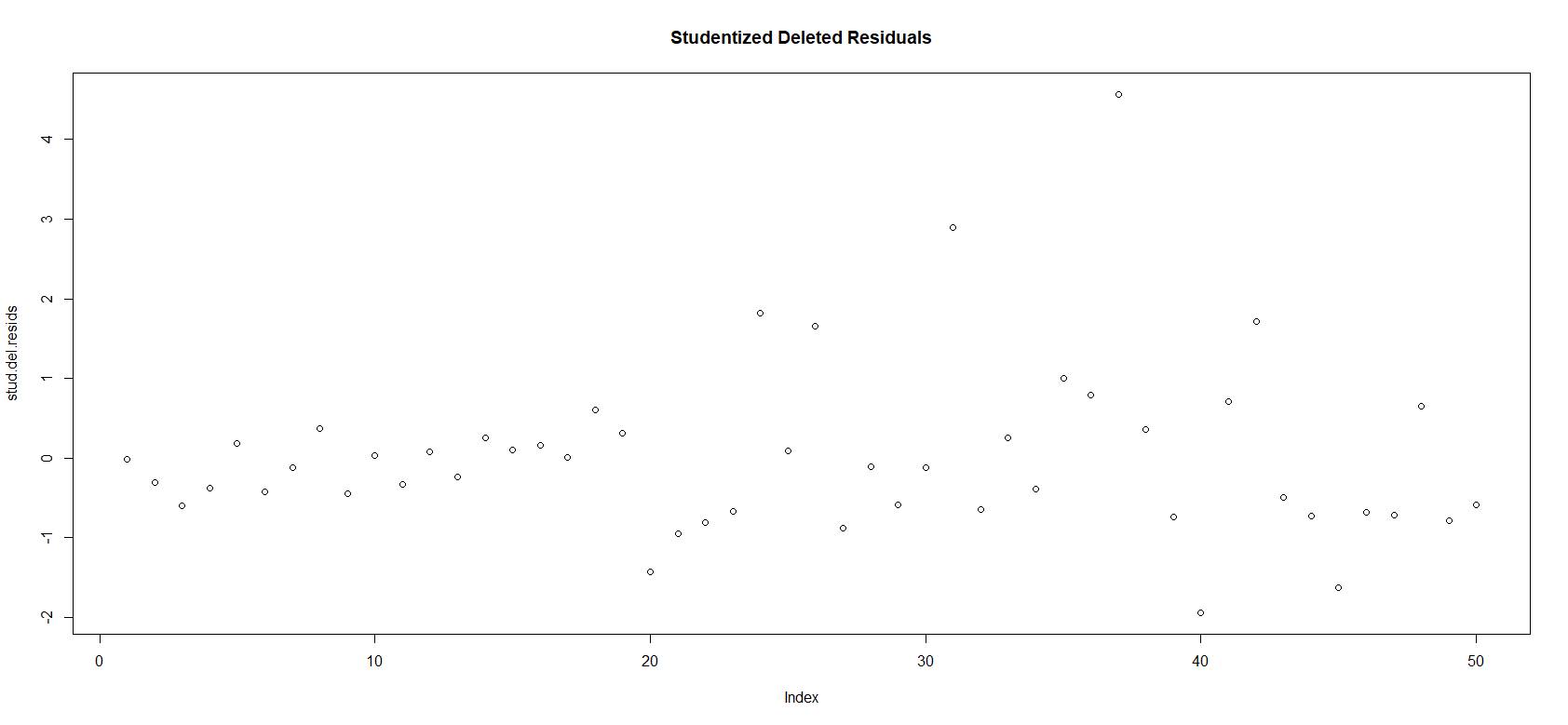
Note that there are 2 observations with studentized deleted residuals that are greater in magnitude than 2. Thus, these observations may be considered outliers. Indeed, both of these observations are apparent in the plot of shooting efficiency against angle and distance given in the data section. The index of the second-largest studentized deleted residual is associated with the outlier in the dependent variable recorded for the 15-distance and 135-degree angle.
A plot of the hat values for the model are given below.
HAT VALUES PLOT
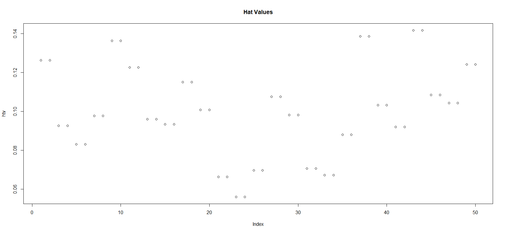
While it is not clear why the hat values plot has two observations at the same positions in the plot (perhaps having something to do with the players taking shots at the same position and angle consecutively), it is clear that none of the hat values is greater than approximately 0.14 < 0.2 and so there is no influential observation (this makes sense given how the data were collected) in the data.
Conclusion
- The purpose of this papaer was to test the hypothesis that two amateur basketball players have greater shooting efficiency when shooting on the side of the basket associated with their shooting arm. A mutiple linear regression model generated, where the independent variable of interest was the side of the basket the shot originated from. Other controls were included in the model to capture the location of the shooter on the court and which shooter was being timed. The results has shown that there was no significant evidence in the data to prove that the shooter’s orientation improved shooting efficiency, with only the parameter associated with the shooter’s distance to the basket being significant. Diagnostic tests indicated that while the residuals deviated from normality and suggested the presence of heteroscedasticity, there was no evidence of autocorrelation in the residuals. The study found no significant multicollinearity among the model predictors, except for one outlying observation.
- Limitations:
-
The sample size is relatively small, consisting of only two amateur basketball players. This limits the generalizability of the results to other populations of basketball players. Additionally, the study only considers shooting efficiency from a fixed location on the court, which may not fully capture the variability in shooting performance that occurs during actual basketball games.
-
The data collection method used in this study may have introduced biases that could affect the accuracy of the results. For example, the choice of moving across the court in a fixed pattern may have influenced the shooting performance of the participants, as they may have become fatigued or experienced other factors that affected their shooting efficiency.
Shreyas Anil A EDA
Changqing (Alex) Yang A Hyp
Freeman Chen A CLT -