quiz1

Study List for Quiz 1: Time Series Analysis §

L1 & L2 Topics Covered: §

---

(a) Objectives of Time Series Analysis §

1. Definition: Understand what is meant by time series analysis.
2. Visualization: How to visualize data measured over time.
3. Key Components:
   • Trend: Long-term movement in data.
   • Seasonality: Patterns that repeat at regular intervals.
   • Cycles: Long-term oscillations without a fixed period.
   • Noise: The random variation in the series.
4. Forecasting: Using previous values to predict future ones.

---

(b) Basic EDA (Exploratory Data Analysis) §

1. Time series plot: Understand how to plot data over time.
2. MA Smoothing (Moving Average):
   • Definition of MA smoothing.
   • Why and how is it used in time series analysis?
3. Classical Decomposition:
   • Breakdown into Trend, Seasonal, and Residual components.
   • Understand how to interpret the components.

---

(c) ARIMA Family for Modeling Time Series Data §

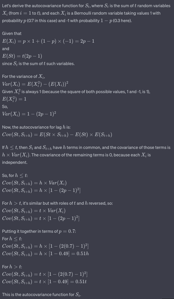
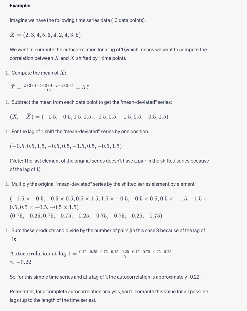
i. Autocovariance and Autocorrelation §

1. Definitions:
   • Autocovariance: How two points at different times but on the same series covary as the time lag, h, changes.
   • Autocorrelation: The linear dependency or correlation between two points on the same series observed at different times with time lag h.
2. Importance: Why are these measurements crucial for time series analysis?

ii. (Weakly) Stationary §

1. Definition: Understand what it means for a time series to be (weakly) stationary.
2. Expected Value Independence: �(��)E(Xt​) is independent of t.
3. Variance Independence: Var(��Xt​) is independent of t.
4. Covariance with lag h Independence: �(ℎ)=cov(��+ℎ,��)γ(h)=cov(Xt+h​,Xt​) is independent of t.
5. Importance: Why stationary time series are easier to model and the significance of modeling stationary series first.

iii. Detecting Stationary Time Series §

1. Time Series Plot: Using visual methods to detect stationarity.

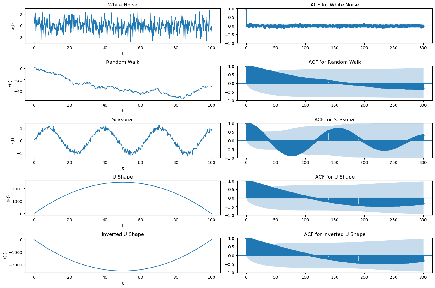
2. Sample Estimate of ACF (ACF Plot):

   • Understand how to read an ACF plot.
   • Recognize patterns in ACF that suggest stationarity.

3. Test for Stationarity: ADF Test (Augmented Dickey-Fuller):

   • Understand the basics of the ADF test.
   • How it’s used to determine if a time series is stationary.

4. Identification:

   • Be able to identify ACF plots for stationary time series.
   • Recognize data with specific patterns suggesting stationarity or non-stationarity.
   • 1. Trend and Seasonality: Non-stationary time series often exhibit trends or seasonality. For instance, an upward trend would result in a high autocorrelation because values that are close in time would be close in value too. Similarly, if there’s a seasonality (like daily, monthly, or yearly patterns), you’d see spikes at regular intervals in the ACF plot.

5. Significance Level: It’s not just the existence of spikes in the ACF plot that matters, but whether those spikes are statistically significant. In many ACF plots, a significance boundary (often represented by horizontal dashed lines) is included. Correlations outside of these boundaries are considered statistically significant.

6. Other Indicators: While the ACF is a useful tool, it’s best used in conjunction with other tests and plots, such as the Augmented Dickey-Fuller test or the KPSS test, to test the stationarity of a time series. Additionally, the partial autocorrelation function (PACF) plot can give insights into the order of autoregression if ARIMA modeling is being considered.

   • dick test:
     • • H0​: The time series has a unit root (i.e., it is non-stationary).
   • �1H1​: The time series does not have a unit root (i.e., it is stationary).
   • If the ADF Statistic is less than the critical value at the 5% significance level (often it’s around -2.86, but it can vary based on sample size), and if the p-value is less than 0.05, then we would reject the null hypothesis and conclude that the series is stationary.

In summary, while a “wavy” ACF plot that doesn’t die out quickly suggests non-stationarity, it’s always a good idea to use multiple methods and tests to confirm your observations and decisions about a time series.