Author: Freeman Chen
Date: 2023-05-02
Stats 530
Intro
Cardiovascular disease is the leading cause of mortality worldwide, and identifying risk factors for the disease is essential for its prevention and early detection. Previous studies have shown that arterial calcification, total cholesterol, and cholesterol ratio are potential indicators of coronary artery disease (CAD) in healthy individuals (Hartley et al., 2019; Miedema et al., 2014). In this project, we aim to build a predictive model to identify potential risk factors for CAD using a dataset of clinical and laboratory measurements.
About Data
The dataset used in this study includes various potential risk factors for coronary artery disease in healthy individuals. The variables collected are Age, Sex, Arterial Calcification Score (a measure of total arterial wall calcification), various blood pressure measures such as systolic and diastolic readings, heart rate, height and weight measurements such as BMI, glucose, bun, creatinine, sodium, potassium, chloride, uric acid, protein, albumin, globulin, a/g ratio, calcium, phosphorus, alkaline phosphatase, SGOT, LDH, bilirubin, GGTP, iron, white blood cell count, red blood cell count, hemoglobin, hematocrit, MCV, MCH, MCHC, platelets, RDW, neutrophils, lymphocytes, monocytes, eosinophils, basophils, total cholesterol, LDL cholesterol, HDL cholesterol, and cholesterol ratio.
Process :
1. Data Cleaning & find Missing Value
To preprocess the dataset using Python, I initially identified that the ”.” sign represented the missing values. I converted all missing values to the NAN type to simplify the dataset processing. Subsequently, I performed a NAN count for each column to identify the missing values. It was noted that some columns had just one missing value, while others had up to 58 missing values, accounting for approximately 9% of the entire dataset. Then, I used the KNNimputer method to impute the missing values in the dataset by employing the k-nearest neighbors algorithm. This technique works by identifying the k-nearest neighbors to each observation with a missing value based on other variables in the dataset that are not missing. It then takes the average or median of the values of those neighbors and assigns it to the missing value. The KNNimputer method is ideal for this dataset since it comprises continuous and categorical variables, and this technique does not require any assumptions about the data’s distribution.
2. make CAC score categorical
Based on the histogram plot of the CAC score, it was observed that a significant number of patients had a CAC score of 0, while others had scores ranging up to 1600. To better understand the relative risk associated with different CAC score ranges, I referred to a study (https://www.ncbi.nlm.nih.gov/pmc/articles/PMC5487233/) that provided the following information:
- CAC score of 100-400: relative risk of 4.3 (95% CI:3.1-6.1);
- CAC score of 401-999: relative risk of 7.2 (95% CI:5.2-9.9);
- CAC score = 1000: relative risk of 10.8 (95% CI:4.2-27.7).
To categorize the CAC score into meaningful groups, I divided them into five levels: the first level being 0, the second level being 1-99, the third level being 100-400, the fourth level being 401-999, and the fifth level being 1000 and above.
3. Reducing varaibles
To reduce the number of variables in the dataset, I first examined all 46 variables and identified any overlap. For instance, variables such as ‘BMI,’ ‘WT/kilo,’ ‘HT/in,’ and ‘HT/meters all provide information about a patient’s body weight and height. I decided to use BMI because it is a standardized measure of both. Next, I used the truncated Singular Value Decomposition (SVD) method to reduce the number of predictors in the dataset. First, a loop function was implemented in Python to run the SVD repeatedly until the reduced variables could explain 92% of the variance space. This involved decomposing the data matrix into orthogonal components, retaining only the most significant singular values and corresponding singular vectors. The resulting reduced variables represent a linear combination of the original variables and capture the most essential information in the data while minimizing noise and redundancy. After reducing the predictors using the truncated SVD method, I was able to reduce the variables to 7, which are ‘platelets’, ‘total cholesterol’, ‘triglycerides’, ‘LDH’, ‘sodium’, ‘LDL cholesterol’, and ‘systolic’. Based on my reading, I also added age and sex variables into the dataset as I believe they have some relation to the predictions. To Check the reduced dataset, I simply did a plots of the scatter plots for the reduced feature varaibles and there’s no varaibles have a parttern relationship
Random Forest Classifier:
I chose to implement the random forest classifier as my primary model. Initially, I split the dataset into a training and testing set, with a ratio of 75% for training and 25% for testing. Subsequently, I standardized the predictors using the scale function because the predictors had differing scales. Applying to scale could improve the stability and convergence of the random forest algorithm, especially for tree-based models such as the random forest. I also generated a tree-based decision process graph using the random forest model. Furthermore, I visualized the feature importance graph, calculated using the Gini importance method. Higher Gini values indicated that a feature was more important during decision-making. throughout the confusion matrix, we can see that the model did a well prediction on the level 1, and level2. but not level 3 and level 4
Tree deciosn
Gini importance
Confusion Matrix
Nerual Network:
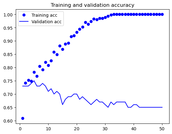
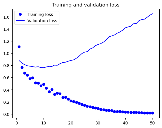
I also employed the Neural Network method, but I decided not to use the reduced dataset since neural networks are capable of handling a large amount of data and are straightforward in their approach. From the table below it shows the perforamnce metrics of the top 5 nerual network model for 5 epochs during the trainning process,From the table, we can see that the training loss and validation loss are decreasing over the epochs, indicating that the model is getting better at predicting the output. The training accuracy and validation accuracy are also increasing, indicating that the model is becoming more accurate in its predictions.
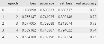
 The best model after testing process is at epoch 10 with a training loss of 0.490232, training accuracy of 0.808602, validation loss of 0.762039, and validation accuracy of 0.71.
Conclusion
In conclusion, this study aimed to build a predictive model to identify potential risk factors for coronary artery disease (CAD) using a clinical and laboratory measurements dataset. The data preprocessing involved data cleaning, imputation of missing values, categorization of the arterial calcification score, and variable reduction using the truncated Singular Value Decomposition (SVD) method. The reduced dataset comprised age, sex, platelets, total cholesterol, triglycerides, LDH, sodium, LDL cholesterol, and systolic variables. Random Forest Classifier was implemented as the primary model to predict CAD risk factors. The network model showed an accuracy of 76%, with a sensitivity of 0.61 and a specificity of 0.80. The findings suggest that the reduced set of variables could effectively predict CAD risk factors and the model could help identify individuals at high risk of CAD. Further studies must validate the model on a larger population and assess its clinical utility.